Welcome to the M_Dart Project of Marinko Laban

(Last updated February 23^rd, 2024)

Introduction

The M_Dart Project

The M_Dart Project is all about writing a book about Global Illumination and implementing a Ray Tracer in Ada 2012 to compute realistic pictures. The working title of the book is The M_Dart Project, with subtitle Computing Global Illumination by Ray Tracing using the Ada 2012 Programming Language

The reasons for starting this project are:

I want to gain experience in the Ada 2012 programming language. I realize C++ is the mainstream ray tracing programming language, but I have affinity with Ada since my days at university, and this is a good-sized project to sink my teeth in.
There is a lot of literature on ray tracing and global illumination. However, it often focuses on the scientific theory and give little practical guidance, or relevant topics (in my perception at least) are left out or only briefly described

So I set myself out to try to develop a ray tracer that is rich in features, and write a book about it that covers both the theory as well as the practical implementation. One of the end goals is to encourage others to write a ray tracer or at least enjoy reading the book. It is my intention to combine theory and practical implementation, in order to help people new to the subject not to get scared by the sometimes complex theory and mathematics. A practical approach, tips & tricks, code snippets and the complete source code will be included to support any readers.

A first attempt to start this project was already in 2009, but due to my professional career and family life, it went dormant for quite a few years. Luckily, in 2014 I found myself again in a position to spend more time on it. I am still juggling time for my career, family and other hobbies. So I made some good progress until 2017, then it slowed down again for the same reason. I still make some progress every now and then, so keep checking back here.

On these pages, I want to keep you up to speed with the scope and progress of the project. I do not intent to distribute my book through here, although I might post some parts of it. In the end, if I ever get there, I intend to publish the book and see if I can get some money out of it, but that is not the prime objective. I intent to distribute the source code, likely in various stages of completion, and in order for you to understand what you might get, let me state the development environment I am using (and which is subject to change over time):

My hardware is a laptop with an Intel© Core™ i9-9980HK CPU @ 2.40GHz, 32 Gb of RAM, and a 1Gb SSD drive
It runs Linux Mint 21.3 Cinnamon
I am using GCC 13.2 (compiled the sources myself) with GNAT and GNAT Studio 23.0. Especially the GNAT Studio IDE is my main platform to develop & test the code
I use LibreOffice to write my book and some of the illustrations. I also use it for maintaining my product backlog, although I don't do full Agile.
I use a variety of tools, like GIMP and Umbrello, to edit some of the illustrations in my book

Since I use Linux freeware (GNU license) to develop the software, I consider the source code to fall under the GNU license as well. So feel free to use it without any warranty, as long as you use it according to the GNU license.

To keep readers informed about the scope and progress of my endeavors, I will start to maintain my product backlog and a simple blog-like diary on this page. Of course, intermediate results as pictures will be posted as well in the gallery.

Feedback

Feel free to feedback any comments or questions you may have. Click here to email me. You can also leave a comment in the GitHub repository with the source code.

Finally, if you want to support me in my work, feel free to buy me a coffee via the button below. It is highly appreciated and helps me to continue my work.

Blog Update: 23 February 2024

Picking up again after couple of years of silence...a few things have been added:

Source code is now available in Git here.
Triangle objects: This as a prelude to triangle-mesh objects
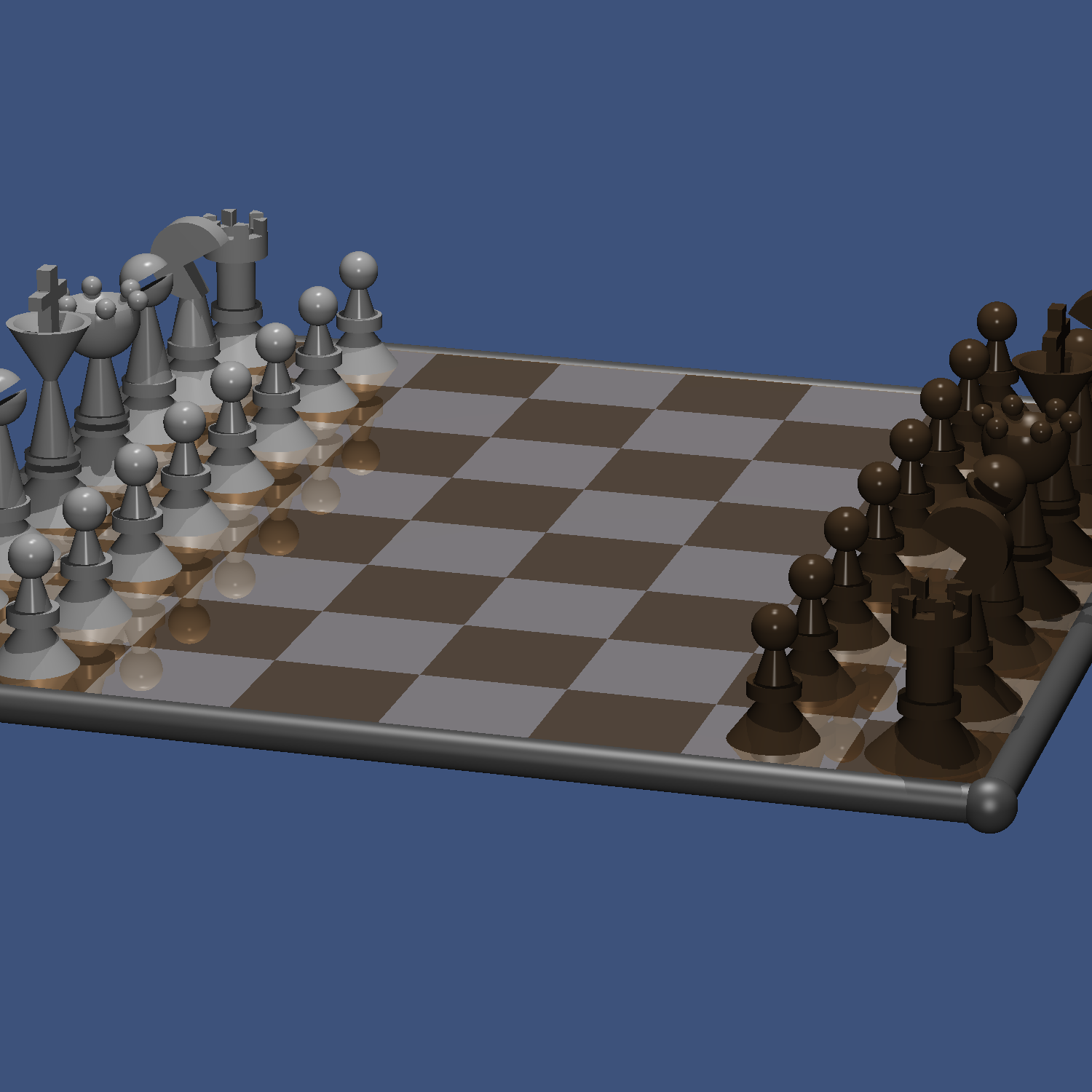
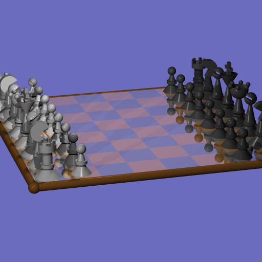
Tone mapping now supporting Reinhard and Reinhard Extended algorithms. These produce better results when it comes to images where RGB values need to be clipped because of high dynamic radiance ranges Below are three images, using Linear, Reingard and Reinhard Extended...you can judge what you like best...but IMHO, the last one is the brightest and most pleasing.

A chessboard model wit linear tonemapping

A chessboard model, where the tiles of the board are somewhat reflective. Sampled with 9 random samples per pixel with a minimal distance of 0.2. Tone Mapping applied is the LINEAR algorithm.

A chessboard model with Reinhard tonemapping

A chessboard model, where the tiles of the board are somewhat reflective. Sampled with 9 random samples per pixel with a minimal distance of 0.2. Tone Mapping applied is the REINHARD algorithm.

A chessboard model with Reinhard-Extended tonemapping

A chessboard model, where the tiles of the board are somewhat reflective. Sampled with 9 random samples per pixel with a minimal distance of 0.2. Tone Mapping applied is the REINHARD-EXTENDED algorithm.

Blog Update: 19 February 2017

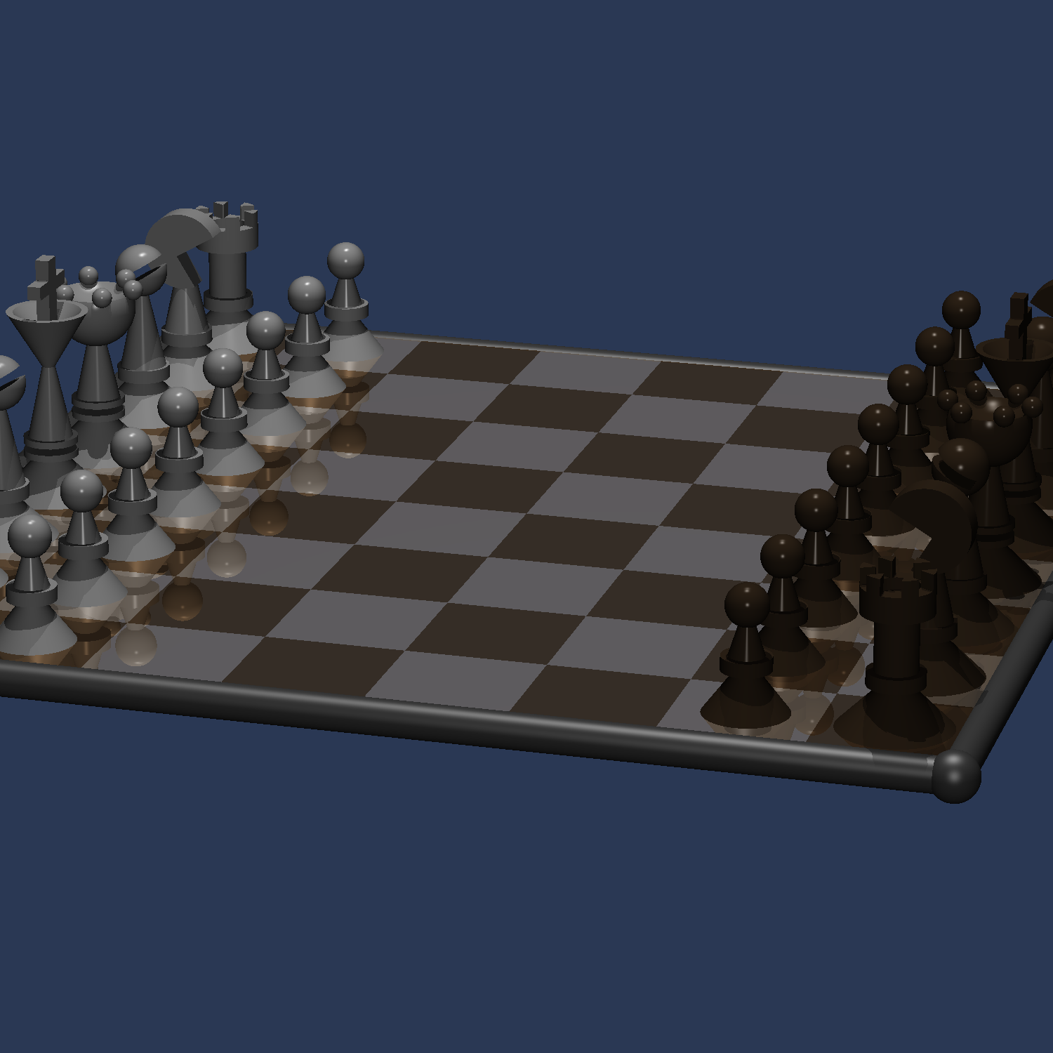
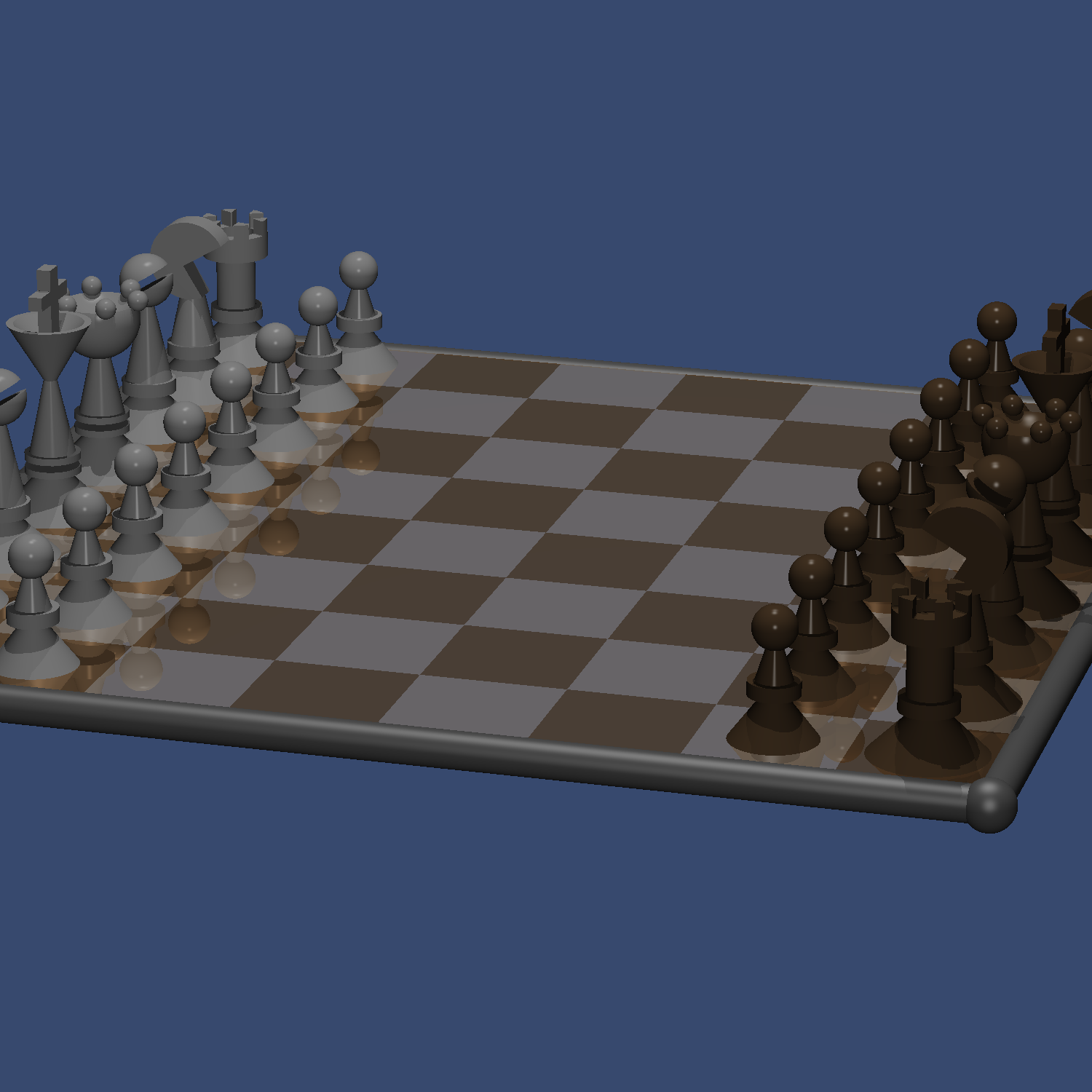
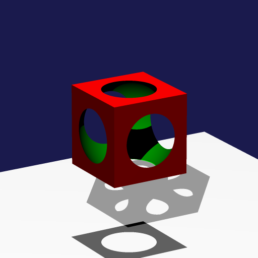
I implemented a simple reflective material, which basically allows you to add reflected light in the ideal direction. Also added a cosine term, so reflections in a more grazing angle to the reflective surface are more prominent, while reflections more perpendicular to the surface are less visible. Also built a more complex scene using CSG, which was worthwhile... the combination of reflection and more complex CSG objects led to two bugs I had to fix: A normal flipped in the wrong direction in my cube intersection code, and the CSG evaluation being cut off too early, resulting in some problems when subtracting an object from another CSG object. The result is rather pleasing though. It' also a good scene to test future acceleration algorithms.

A chessboard model, where the tiles of the board are somewhat reflective

A chessboard model, where the tiles of the board are somewhat reflective. Sampled with 9 regular samples per pixel.

Blog Update: 22 January 2017

I implemented a Phong material this period. At first it appeared to be straightforward, but with low, odd-powered parameters, it turned out I made a mistake in my code. Hence it took a bit longer to complete it, but finally it seems all to be working correctly. I do not enforce energy balance (i.e ambient + diffuse + specular reflection factor = 1.0), so I can actually be a bit more flexible with the materials, although physically not per se realistic. Below are some results...

9 red spheres, where diffuse + specular reflection spectrum = 1.0. Diffuse is increasing, and specular is decreasing

9 red spheres, where diffuse + specular reflection spectrum = 1.0. Diffuse is increasing, and specular is decreasing. The spheres get more dull from left to right and top to bottom. Sampled with 25 regular samples per pixel.

9 red spheres, where the power is increasing, to produce sharper highlight, giving the spheres an increasing reflection look

9 red spheres, where the power is increasing, to produce sharper highlight, giving the spheres an increasing polished look with a higher power. Sampled with 25 regular samples per pixel.

9 red spheres, where only the diffuse spectrum is increasing, and the specular spectrum is a constant WHITE

9 red spheres, where only the diffuse spectrum is increasing, and the specular spectrum is a constant WHITE. The spheres appear less dark, or less glass-like. Sampled with 25 regular samples per pixel.

Blog Update: 10 January 2017

Finally upgraded to newer hardware...see the revised spec above...Ran some tests and it is quite a bit faster, as expected. I have updated the times in the gallery accordingly. The first image went down from >5 mins to >1 mins, which is not bad at all. Also added some extra stats for CSG evaluation and length of the ShadePoint list. The CSG evaluation counts the number of times a CSG evaluation has been called on an object. As this is a recursive evaluation, even a simple CSG object like the ones in the previous posting will generate multiple CSG evaluations on average per ray intersection (ShadePoint). This is because my code evaluates upwards from any primitive object hit in the CSG tree.

Blog Update: 23 December 2016

Wow...this period was a challenge...I changed the planning a bit and started to implement Constructive Solid Geometry (CSG) a bit earlier. This turned out to be a bit more complex... Especially getting it to work with shadows was a bit of a struggle, but I finally got it working. See below for some example pictures.

The intersection between a cylinder and a sphere substracted from another sphere

The intersection between a cylinder and a sphere subtracted from another sphere, sampled with 9 samples per pixel, regularly distributed in a 3x3 grid.

The UNION between a red cube and a green sphere

The UNION between a red cube and a green sphere.

The INTERSECTION between a red cube and a green sphere

The INTERSECTION between a red cube and a green sphere.

The DIFFERENCE between a red cube and a green sphere

The DIFFERENCE between a red cube and a green sphere.

Blog Update: 12 November 2016

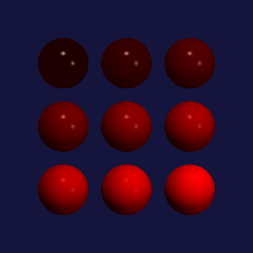
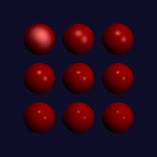
This period I did some more work on the Filter code. I added skeleton code for Filter classes, and implemented a Box filter (all samples have an equal weight) and a Multi Stage Filter (the pixel is divided in a grid of 4x4 squares. The samples in each square are box-filtered, then the 16 square samples are box filtered). I also built a test scene containing a row of very thin cones, in alternating yellow and red colours. The cones are very thin and close to each other, such that their tops are much smaller than a pixel. They are also spread evenly but with a distance that is not matching the pixel distance. In other words, in pixel 1 the cone top may be in the centre, but in pixel 2 the top is slightly more to the right...and so forth... Therefore, rays will easily miss the tops of the cones, even with multiple rays per pixel. This scene is derived from Robert L. Cook's article "Stochastic Sampling in Computer Graphics". Below are a number of images where a random distribution of samples is compared with regular distribution.

Red and yellow cones, 1 sample per pixel, through the pixel centre

Red and yellow cones, 1 sample per pixel, through the pixel centre. Note how the cone heights seem to alternate in a saw-like pattern, which is caused by the rays missing the cones in a regular pattern. The cones therefore seem to alternate in height in a regular fashion. This is an extreme form of aliasing.

Red and yellow cones, 1 sample per pixel, randomly positioned

Red and yellow cones, 1 sample per pixel, randomly positioned in the pixel. Note how the saw-like patterns are now replaced by a grainy pattern. In fact, the aliases in the previous image are now replaced by noise. Although the noise is unpleasantly noticeable (there appear to be holes in some cones), at least the cones seem to be of a similar height.

Red and yellow cones, 16 samples per pixel, regularly distributed

Red and yellow cones, 16 samples per pixel, regularly distributed. Note how the regular saw-like patterns are still noticeable, although smaller in size. The 4x4 samples reduces the aliasing, but it is still there.

Red and yellow cones, 16 sample per pixel, randomly positioned, box filtered

Red and yellow cones, 16 sample per pixel, randomly positioned, box filtered. Note that the grainy noise is now much less noticeable, and the cones are pretty even in height.

Red and yellow cones, 16 sample per pixel, randomly positioned, multi-stage filtered

Red and yellow cones, 16 sample per pixel, randomly positioned, multi-stage filtered. You probably need to zoom in and compare with the previous picture, but you can see that this image is a bit less grainy than the previous one. The multi-stage filter avoids "cluttered sample positions" to have a biased influence on the pixel colour.

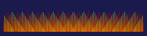
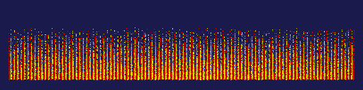
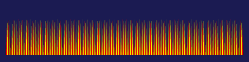
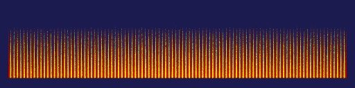
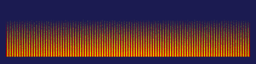
Obviously, you can debate which picture is nicer to look at. Arguably, people may find the regular samples images prettier, but it is not about how pretty an image may be. It is all about how accurate it is. So in my mind, the saw-like patterns may be pleasing to see, but they are not accurately displaying the cones, which are all of the same height. Therefore, replacing aliases by noise will bring more realism in your images...if you bring the noise levels down to an acceptable level, by using more samples and appropriate filtering, you will get both realistic as pleasing images. I ran the images above also with higher sampling rates (up to 32x32 samples). Around 8x8 random samples, the noise becomes barely noticable, while the regular samples still show saw-like patterns and moire patterns.

Blog Update: 13 August 2016

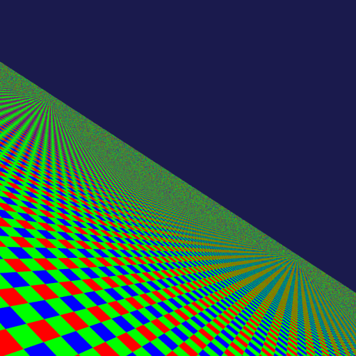
This period I did some more work on the Sampling code. I added skeleton code to generate randomly distributed samples, but now with a minimal distance. This gives a more evenly distributed set of samples compared to pure random. I did not implement any specific filtering yet. All samples equally influence the pixel colour, which effectively means a box filter is used. A few examples of another checkered plane...note that the colours blend into yellow and light blue in the distance, although all squares are really just pure red, green or blue.

Checkered plane, 25 regular samples per pixel

A checkered plane, sampled with 25 samples per pixel, regularly distributed in a 5x5 grid. Note the arc-like patterns near the horizon, caused by aliasing, even with 25 samples.

Checkered plane, 16 random sample per pixel

A checkered plane, sampled with 16 samples per pixel, randomly distributed with a minimal distance of 0.2 on a unit square. Note that the arc-like aliases are now replaced by noise. Personally, I think this picture looks better, despite the lower sampling rate.

Blog Update: 10 July 2016

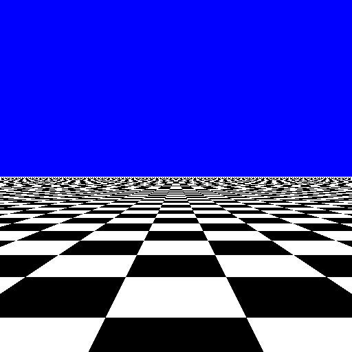
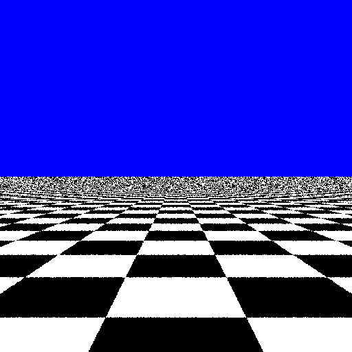
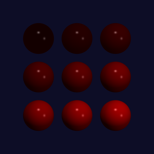
This weekend I worked on the Sampling Chapters. Part of this is showing how different sampling techniques impact quality of an image. To demonstrate this, see the images below of a checkered plane.

Checkered plane, 1 regular sample per pixel

A checkered plane, sampled with one sample per pixel through the centre of the pixel. Note the strong arc-like patterns near the horizon, caused by aliasing.

Checkered plane, 1 random sample per pixel

A checkered plane, sampled with one sample per pixel randomly. Note that the arc-like aliases are now replaced by noise.